How the Rent Relief Act of 2019 Varies with Income and Location

We show the impact on different households of the tax credit bill introduced by then-Senator Kamala Harris.

Kamala Harris on Friday released her economic plan, including an expanded Child Tax Credit we analyzed on Saturday. Absent from the housing portion of her plan was legislation she introduced in 2018 and 2019 as a Senator: the Rent Relief Act (RRA), a refundable tax credit based on income, rent paid, and local housing costs. In this post, we use the PolicyEngine model to explore its effects on different household types, and how it situates with other tax and benefit programs. We focus on a typical example, as well as two ends of the credit’s generosity spectrum, based on local housing costs, at which the bill caps countable rent.

While Harris introduced the RRA in the Senate in 2018 and then 2019, the bill dates back to 2017 and continues to be active:

• 2017: Rep. Joseph Crowley (D-NY) introduced the initial version with eight cosponsors.

• 2018: Rep. Scott Peters (D-CA) reintroduced it in the House; Sen. Kamala Harris introduced a Senate companion bill.

• 2019: Sen. Harris and Rep. Danny Davis (D-IL) reintroduced it in the Senate and House, respectively, reducing the maximum rent from 150% to 100% of fair market rent.

• 2022: Rep. Davis and Sen. Raphael Warnock (D-GA) reintroduced the bill.

• 2023: Rep. Davis reintroduced it without a Senate companion.

The bill has not changed since 2019, and all 25 cosponsors in the latest House bill are Democrats.

The RRA establishes a refundable tax credit based on household income, rent paid, and local housing costs. The bill defines local housing costs from Small Area Fair Market Rents (SAFMRs), which HUD sets at the 40th percentile of rents in each ZIP code, broken down by the number of bedrooms. HUD publishes these SAFMRs annually, and this spreadsheet shows them for 2024.

Key features of the credit:

• Covers a percentage of rent exceeding 30% of the household’s gross income

• Percentage decreases as income increases, according to the following schedule: 100% for incomes up to $25,000, 75% for incomes over $25,000 but not over $50,000, 50% for incomes over $50,000 but not over $75,000, 25% for incomes over $75,000 but not over $100,000, 0% for incomes over $100,000

• Thresholds are $25,000 higher in areas that use SAFMRs instead of FMRs (which HUD defines at the metro level) for the Housing Choice Voucher program

• Uses SAFMRs to determine maximum allowable rent for credit calculation

• Alternate rules for residents of public housing (not modeled in this piece)

• Credit is refundable, meaning it can exceed the amount of taxes owed

This structure creates a varying impact on households depending on their income, rent, and location. The subsequent sections will explore these impacts through specific examples.

We will examine three examples to illustrate the Rent Relief Act’s effects on different household types across various income levels. These examples will focus on a typical household, as well as two households at opposite ends of the credit’s generosity spectrum based on local housing costs.

Consider a single parent with two children living in ZIP code 75459 in Sherman-Denison, Texas, an area with SAFMRs close to the median that does not use SAFMRs for the HCV program. Suppose this household pays $1,500 per month in rent for their three-bedroom home, less than the $1,590 per month SAFMR. Suppose further that they earn $40,000 per year. The credit would cover 75% of the difference between their rent ($18,000) exceeding 30% of their income ($12,000), or 75% of $6,000 which is $4,500.

We can see this visually by displaying the credit with earnings, showing the steps at $25,000 and $50,000, and their ineligibility at $60,000 income (30% of which is $1,500 per month).

Figure 1: Rent Relief Act for a Sherman-Denison, Texas 3-bedroom

The steps at $25,000 and $50,000 income create cliffs. Combined with other tax and benefit programs, the household would have a lower net income if earning between $25,000 and $48,000.

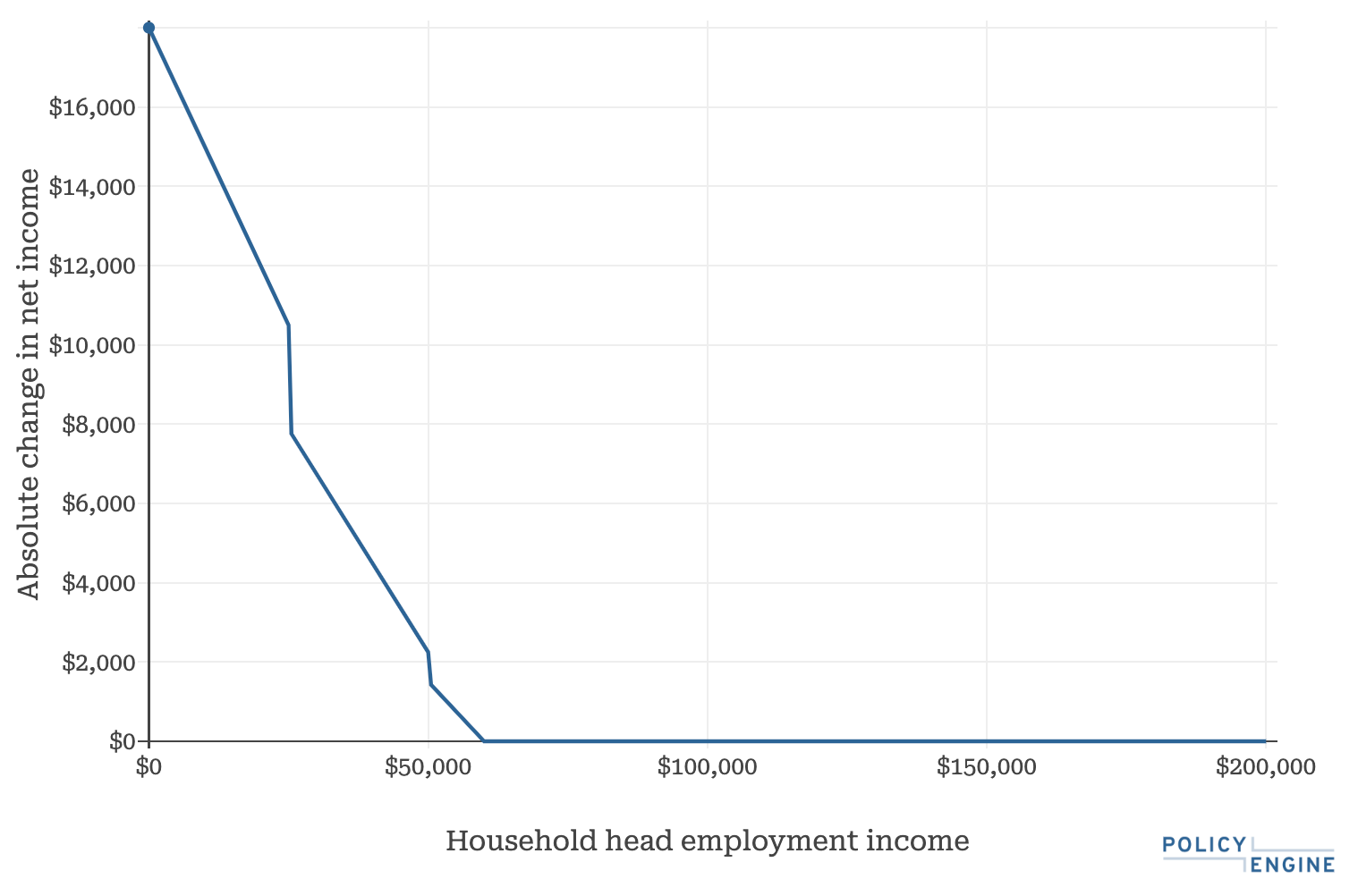
Figure 2: Rent Relief Act Impact on a Single Parent of Two in a Sherman-Denison, Texas 3-bedroom

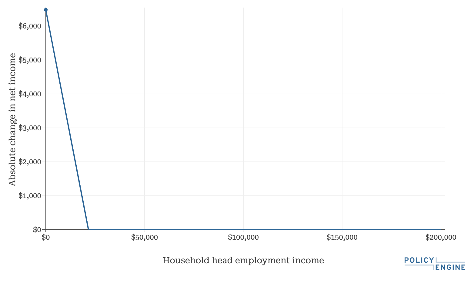
HUD has designated the country’s lowest SAFMR as studios in a set of ZIPs in central Missouri, at $540 per month. Consider an individual living in a studio apartment in this area paying $600 per month:

• If their income is $0, they would receive the full $540 per month ($6,480 annually) as a credit.

• As their income increases, the credit phases out at a 30% rate.

• At $21,600 annual income (30% of which is $540 per month), they would no longer be eligible for the credit.

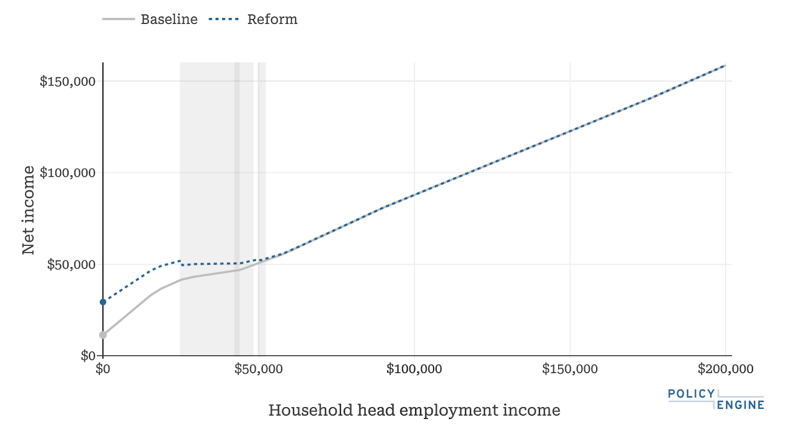
Figure 3: Rent Relief Act for a Missouri Studio

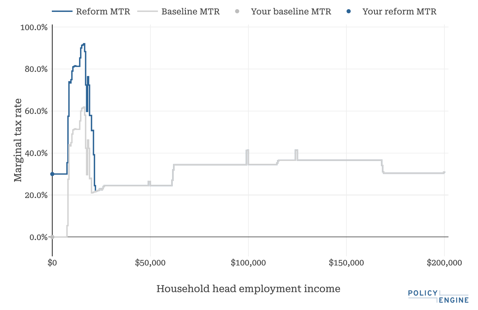
As their baseline marginal tax rate ranges from 0% to 62% in this range, the RRA increases it to between 30% and 92%.

Figure 4: Rent Relief Act Marginal Tax Rate Impact on a Single Person in a Missouri Studio

The country’s highest SAFMR is 4bd in several areas in San Diego: $6,960. This is also an area where SAFMR is used for HCV, raising RRA income thresholds by $25,000.

Consider a married couple with three children paying at least $6,960 per month in rent in a 4bd home in one of these areas. If they have no income, they will receive the full $6,960 per month, or $83,520 per year. That will phase out at a 30% rate, until they earn $50,000, at which point the credit covers 75%, rather than 100%, of the gap between rent and 30% of their income. It then steps down again at $75,000, $100,000, and finally $125,000 income at which point they become ineligible.

Figure 5: Rent Relief Act for a San Diego 4-bedroom

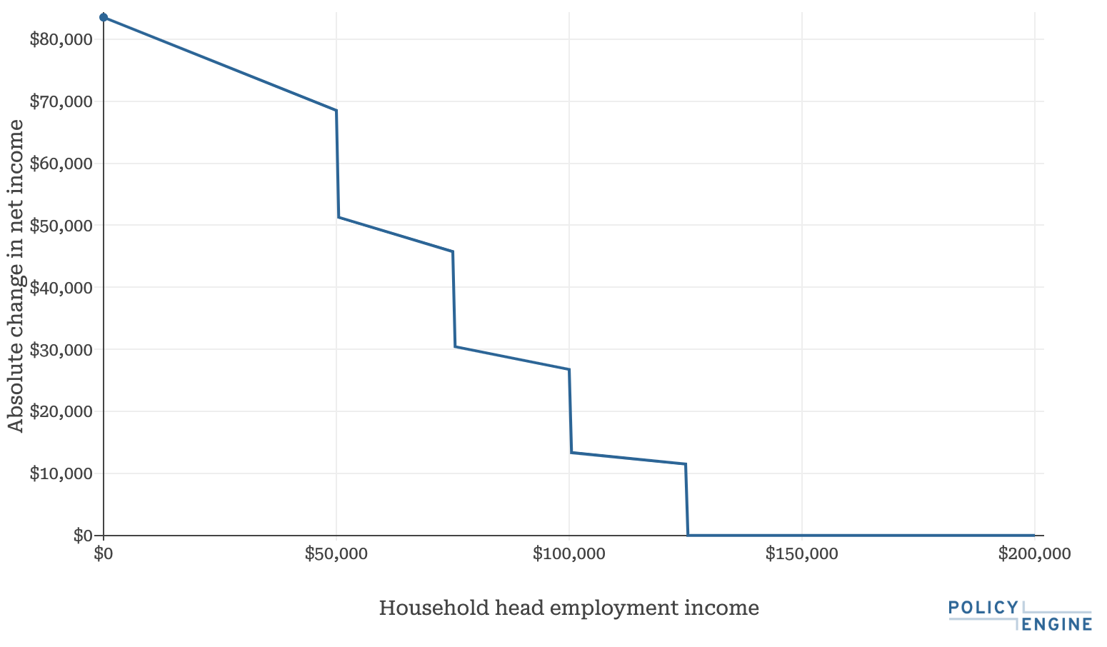
While the credit phases out at a 30% rate for any segment, it creates a higher average marginal tax rate over the full earnings range due to the steps: by reducing the credit from $83,520 to $0 over the earnings range $0 to $125,000, it adds 67 percentage points to their marginal tax rate.

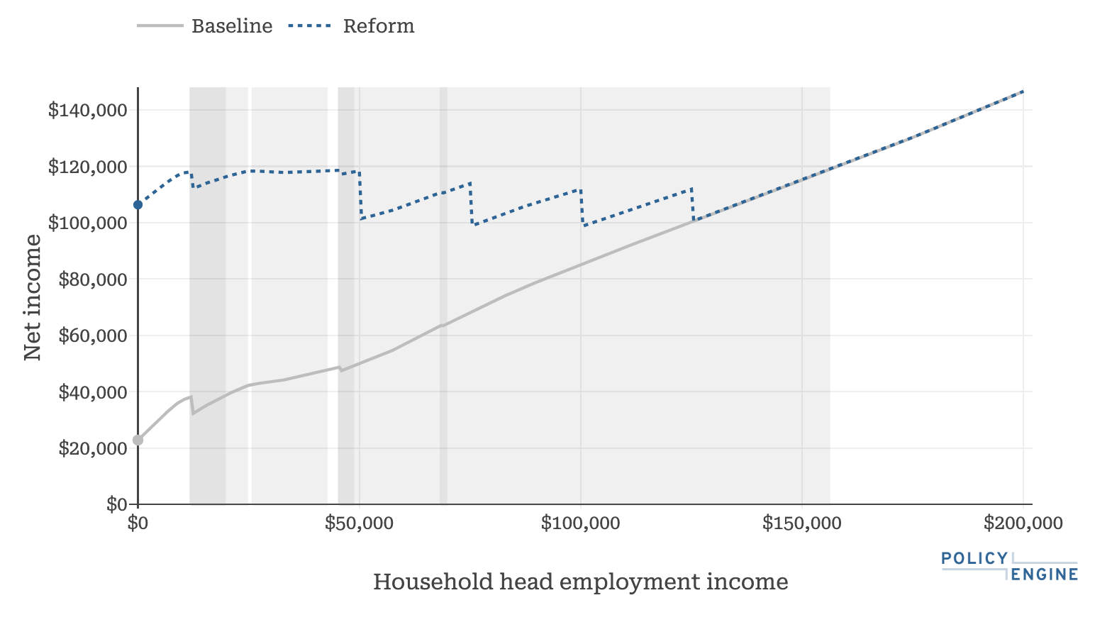
Stacking the credit atop other tax and benefit programs for this household reveals its effect on cliffs. Accounting for state and federal income taxes, and benefits like the Supplemental Nutrition Assistance Program, the household faces a baseline average marginal tax rate of 38% from $0 to $125,000: they receive $22,817 at zero earnings and $100,351 at $125,000. The RRA thus increases their MTR to 105% over this range; their net income is $106,337 at zero earnings and $100,351 at $125,000.

Figure 6: Rent Relief Act Impact on a Couple with Three Children in a San Diego 4-bedroom

It’s worth noting that the bill does not set a maximum number of bedrooms based on household size, unlike the Housing Choice Voucher program. This means the San Diego example could theoretically apply to a single individual living in a four-bedroom home.

To illustrate how the Rent Relief Act affects different household types across various income levels, we can compare the credit amount for all three example households as a function of income:

Figure 7: Rent Relief Act Credit for Selected Homes

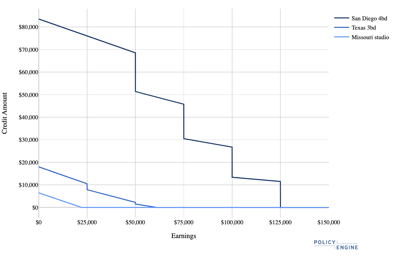
This chart demonstrates several key features of the Rent Relief Act:

• Initial Credit Amount: The San Diego household starts with the highest credit due to the high local SAFMR, followed by the Sherman-Denison household, and then the Missouri household.
• Phase-Out Rates: All households experience the same 30% phase-out rate between income thresholds, as evidenced by the parallel slopes in these regions. Income Thresholds: The San Diego household’s income thresholds are $25,000 higher than the other two due to the use of SAFMRs for the Housing Choice Voucher program in that area.
• Credit Duration: The San Diego household remains eligible for the credit at much higher income levels compared to the other two households, due to both the higher initial credit amount and the elevated income thresholds.
• Cliff Effects: All three households experience cliff effects at their respective income thresholds, where the credit amount drops sharply over a small increase in income.
• Zero Credit Point: The income level at which each household becomes ineligible for the credit varies significantly, from $21,600 for the Missouri household to $60,000 for the Sherman-Denison household, and $125,000 for the San Diego household.

This comparison illustrates how the Rent Relief Act’s impact varies based on local housing costs and whether an area uses SAFMRs for the Housing Choice Voucher program. It also highlights the uniform nature of the phase-out structure across different household types and locations, while showing how this structure interacts with varying rent levels to produce different outcomes for each household.

The Rent Relief Act (RRA) of 2019 proposes a refundable tax credit that would have varying impacts on renter households across the United States. This analysis demonstrates several key aspects of the bill’s potential effects:

• Geographic Variation: The credit’s value differs based on location due to its reliance on Small Area Fair Market Rents (SAFMRs). As shown in the examples, the maximum credit ranges from $540 per month in low-cost areas of Missouri to $6,960 per month in high-cost areas of San Diego.

• Income-Based Phase-Out: The credit’s structure, with its stepped percentage reductions at specific income thresholds, creates a set of incentives that vary with household income. This design leads to cliff effects at $25,000 income increments, where increases in earnings can result in decreases in credit amount.

• Interaction with Existing Programs: When combined with other tax and benefit programs, the RRA can alter marginal tax rates. In some cases, as demonstrated in the San Diego example, this can lead to situations where households may face high marginal tax rates or see their net income decrease as their earnings increase.

• Rent-to-Income Ratio: The credit’s design targets households paying more than 30% of their income in rent, with the largest benefits going to those with the highest rent burdens relative to their incomes.

• Potential Locational Incentives: By tying the credit amount to local rent levels, the RRA could potentially influence household decisions about where to live.

• Flexibility in Unit Size: Unlike some housing assistance programs, the RRA does not limit unit size based on household composition.

These features of the Rent Relief Act illustrate the various factors involved in designing housing assistance policies that aim to address affordability issues across diverse housing markets and household types. The bill’s impacts would likely vary depending on local housing costs, household incomes, and interactions with existing social programs.

In modeling the program’s effects, it is important to consider these incentive effects. Given our recent work integrating labor supply responses in microsimulations, we plan to examine the literature around migration to incorporate this into future analysis. This approach will allow for a more comprehensive understanding of how the RRA might influence both employment decisions and geographical mobility.

Further research could explore the potential effects of the RRA on rental markets, including possible impacts on rent levels and housing supply. Additionally, analysis of the bill’s budgetary implications and its effects on poverty rates and housing stability across different demographic groups could provide insights for understanding the full scope of the proposed legislation.

max ghenis
PolicyEngine's Co-founder and CEO

© 2025 PolicyEngine. All rights reserved.